The blog of Alvaro Boiero

"Live as if you were going to die tomorrow. Learn as if you were going to live forever" Mahatma Gandhi

The blog of Alvaro Boiero

geo

"Live as if you were going to die tomorrow. Learn as if you were going to live forever" Mahatma Gandhi

Seismic response spectra: the intersection between geotechnical engineering and seismic-resistant design of structures

The seismic response spectrum is a fundamental tool to perform the seismic-resistant design of most structures. However, the physical meaning of the response spectrum is often unknown to many professionals, who simply apply what is established in the current standards. Do you want to learn more about this important design tool? Continue reading this post...

Content

The concept of seismic response spectrum

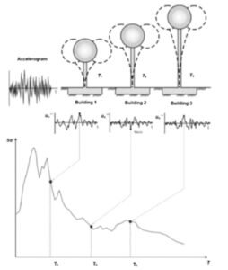
First, let's review the concept of seismic response spectrum. To do so, it is important to mention that seismic movements are recorded through accelerograms, which represent the variation of the acceleration induced by an earthquake at the site where the seismological station is installed, during the time the event lasts.

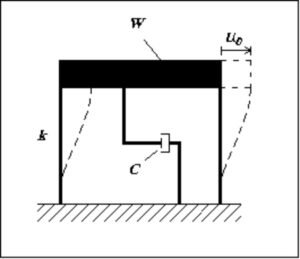
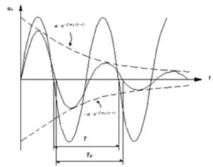
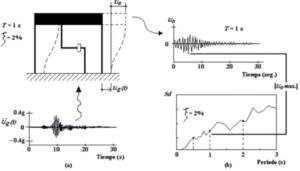
Thus, from the record reflected in the accelerogram, one can calculate, with a simple numerical integration, what is the maximum acceleration that would be induced in a simple linear oscillator with specific damping ζ and a natural period T. The plot of these maximum accelerations as a function of period T, for an assumed simple oscillator with a given damping, constitutes the acceleration response spectrum.

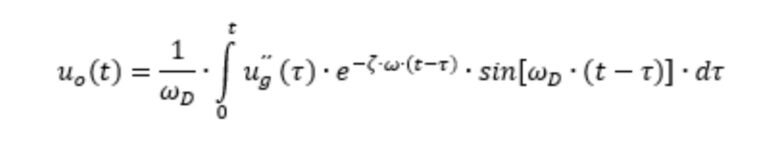
Likewise, by means of a relatively simple mathematical treatment of the accelerogram, the signals corresponding to velocities and displacements can be obtained, and the corresponding response spectra can also be generated. Figure 1 shows an example of the displacement, velocity and acceleration response spectra combined in a single graph.

Figure 1 Seismic response spectra for a damping ζ = 2%. El Centro earthquake, 1940 (Source: available at https://boffi.github.io/dati_2018/10/handout_e.pdf).


Accordingly, the response spectrum makes it possible to directly determine displacements, velocities and maximum accelerations that a seismic movement would cause in structures similar to simple linear oscillators, and in the different modes of structures similar to multiple linear oscillators. Hence, the response spectrum is a fundamental tool for the seismic-resistant design of most structures.


In some specific geotechnical problems, such as soil liquefaction or earthwork stability, where modeling with single or multiple linear oscillators is not appropriate, the use of the response spectrum to characterize the seismic motion is less frequent. However, the analysis of the modification of seismic motion as it propagates through the ground (a very important topic for the study of structural dynamics) is usually performed using response spectra (Jiménez Salas, 1980).

Single degree of freedom systems (1DFS)

The simplest possible structural system is a one-degree-of-freedom system. This can be exemplified by a rigid slab or roof, of weight W, supported by axially rigid columns of negligible mass, with finite bending stiffness k, embedded in its base. This system has, in addition, a damping C that allows energy absorption in the elastic range (Newmark & Rosenblueth, 1971). Such a system is shown in Figure 2.

Figure 2 A damped 1DFS (Source: Grases, 1997).

A very important concept in this type of systems is the critical damping fraction ζ. Basically, ζ affects the free vibration by reducing it. Since ζ = C / CCRIT, when the damper constant C is equal to or greater than CCRIT, the system does not oscillate by moving it, or by making it acquire velocity and letting it move freely, but gradually returns to its original undeformed state, which it recovers after an infinitely long time. When the constants of the damper are less than CCRIT, the system tends, oscillating, to that state (Newmark and Rosenblueth, 1971).


What does this mean from a practical point of view? Figure 3 may help to answer this question. It shows two plots: one corresponding to a system without damping, which oscillates with the same amplitude for a certain time t; and the other representing a system with damping D, in which the amplitude decreases for increasing values of t.

Figure 3 Free oscillations in a simple system (Source: modified from Newmark & Rosenblueth, 1971).

Basically, if we think in ductile structures designed to resist seismic movements, they present a behavior that follows this pattern.

Obtaining seismic response spectra

Given an oscillator with a viscous damper, the seismic action on the oscillator is simulated by ground displacements, velocities, and accelerations, denoted by ug(t), u'g(t), and u''g(t), respectively. Therefore, the oscillator will undergo relative displacements, relative velocities, and absolute accelerations. The dynamic equilibrium condition of the oscillator mass will be:

Given the history of ground accelerations u''g, the above equation depends on the damping ζ and the circular frequency  (or period T) of the undamped system. The solution of this equation can be written in terms of the Duhamel integral (Grases, 1997), as follows:

For ζ ≤ 0.20 the value of D is, for practical purposes, equal to the value of . The maximum value of the displacement obtained for a particular period is the ordinate of the relative displacement spectrum; repeating the calculation for different periods allows obtaining the envelope of the maximum displacements, which constitutes the relative displacement spectrum (Sd) for a selected damping ζ (Wiegel, 1970). The process is summarized in Figure 4.


The product ω.Sd has units of velocity and is related to the maximum strain energy stored in the system during the response. Thus, the Spv vs. T plot is called the pseudo-velocity response spectrum (Grases, 1997).

Figure 4 Obtaining ordinates of the relative displacement spectrum Sd. (a) Oscillator of T = 1 s and ζ = 0.02 subjected to seismic vibrations; (b) Selection of the spectral ordinate Sd (Source: modified from Grases, 1997).

For most seismic motions, the pseudo-velocity and relative velocity do not differ much. However, for high periods there may be a marked difference (Wiegel, 1970).


On the other hand, the product ω2.Sd represents the ordinate of the pseudo-acceleration response spectrum. The graph Sa vs.T is called pseudo-accelerations response spectrum, and its similarity with the absolute accelerations response spectrum is not valid for very small periods, nor for very long periods (Grases, 1997).


It is important to point out that the spectra obtained according to the procedure briefly described above, depend on the stratigraphic and dynamic properties of the soil. Thus, considering that seismic waves propagate through a ground that has a certain characteristic period, a maximum of amplification will be found when this period resembles the predominant period of the seismic event. And the same will occur in structures that present vibration periods similar to those of the ground, producing the phenomenon of resonance.


As can be seen from the above, it is essential to select design accelerograms representative of the seismic hazard of the study area. In future posts we will go deeper into this topic, but it is something to keep in mind.

Physical interpretation of seismic response spectra

In order to understand the physical phenomenon of the response spectrum in a simple way, we can assume a city with buildings of different heights, each of which has a certain fundamental period of vibration. Therefore, it is possible to represent these buildings by inverted pendulums, which have the same periods. In this way, the city would be represented by a series of pendulums of different periods and masses.


If the action of an earthquake with a predominant period is assumed, taking into account that each pendulum has its own period of vibration, the ground will strongly excite the pendulums that coincide close to the periods of the ground. The other pendulums will be little excited, and some will pass the seismic movement without being significantly affected.


If an acceleration meter were placed at the center of mass of each pendulum, the amplification of the acceleration suffered by the center of mass with respect to the ground acceleration would be found. By plotting these values graphically, the response spectrum would be formed.


Figure 5 illustrates the above reasoning


Figure 5 Simple interpretation of the response spectrum (Source: modified from Zeevaert, 1995).

From the above, it is evident that the response of buildings in a given region where they are constructed, will depend on both the fundamental period of the soil and the period of the structure itself.


So far this post on seismic response spectra, which represent a sort of intersection between Geotechnical Engineering and Structural Engineering. Later on we will deal with the topic of seismic hazard, which is fundamental to analyze the seismic response of the ground in a given area.

References

  • Boffi, G. (2018) “Earthquake excitation”. Politecnico di Milano. Available at https://boffi.github.io/dati_2018/10/handout_e.pdf
  • Grases, J. (1997) “Acciones sísmicas, espectros de respuesta, peligrosidad y zonificación”. Publicado en el libro Diseño sismorresistente. Especificaciones y criterios empleados en Venezuela. Academia de Ciencias Físicas, Matemáticas y Naturales. Caracas, Venezuela.
  • Jiménez Salas, A. (1980) “Geotecnia y cimientos III”. 2da. Edición, Editorial La Rueda. Madrid, España.
  • Newmark, N. y Rosenblueth, E. (1971) “Fundamentals for Earthquake Engineering”. Prentice Hall. USA.
  • Wiegel, R. (1970) “Earthquake Engineering”, Prentice-Hall. Englewood Cliffs, New Jersey, USA.
  • Zeervaert, L. (1995) “Diseño sismo-geodinámico de cimentaciones”. Facultad de Ingeniería de la UNAM, División de Estudios de Post-grado. México D. F., México.

2020 - geo blog All rights reserved

en_US