
The hydrometer test for soils
The hydrometer test is essential to estimate the particle size distribution of soils passing through the #200 sieve. From this test, it is possible to determine the proportion of silts and clays in a soil sample, information of utmost importance to predict the behavior of the ground. Do you want to learn more about the basics of this test and its application in Geotechnical Engineering? Then, continue reading this post...
Content
Fundamentals of hydrometer test for soils
Since particle size analysis by sieving is impractical for particle sizes below 0.076 mm (corresponding to the aperture of the #200 sieve), the hydrometry test can be used for fine soils.
In hydrometric analysis, a soil sample is dispersed in water, and the solution is then left to stand, so that the soil particles settle out individually. From a practical point of view, it is assumed that the particles are spherical, and that the process follows Stokes' Law.
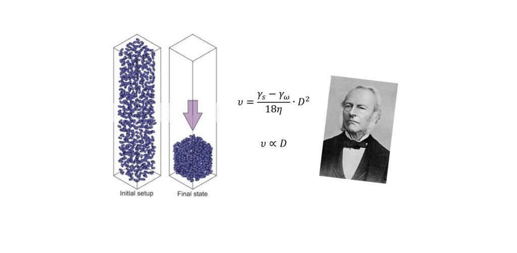
Figure 1 The Stokes´ Law.
This law, enunciated around 1850, states that there is a direct relationship between the settling velocity of a particle in a fluid and the particle size. Adapting this principle to Soil Mechanics, this means that the settling velocity of solid particles in a soil sample is directly proportional to their size, and that as time passes, larger particles will settle faster than smaller ones. Based on the above, it is possible to obtain the value of a certain equivalent diameter of a sphere, whose specific gravity is the same as that of the soil particles whose particle size distribution is being analyzed, during a sedimentation process.
The hydrometer is a measuring instrument, developed from the investigations of the British chemist William Nicholson at the end of the 18th century, with which it is possible to measure the concentration of a soil-water suspension at a certain depth L. Thus, it is possible to estimate the diameter of the particles that settled below L at a time t from the beginning of the test, based on Stokes' Law mentioned above.
Basically, the hydrometric test consists of preparing 1,000 mL of a solution of approximately 50 g of material passing through the #40 sieve, shaking it (in order to achieve a certain homogenization), and then leaving it to settle so that the particles settle. During this process, readings are taken with the hydrometer at different times (usually at 15 s, 30 s, 1 min, 2 min, 4 min, 15 min, 30 min, 1 h, 2 hs, 4 hs, 8 hs, 16 hs, and 24 hs), and then the corresponding calculations are made, following the aforementioned principles. Figure 2 illustrates the process briefly described so far.

Figure 2 Fundamentals of hydrometer test
It is worth mentioning that the ASTM 152 H hydrometer is used in Soil Mechanics laboratory. Also, in order to limit the formation of floccules between the soil particles, a dispersing agent, usually sodium hexametaphosphate, is added to the solution. In this way, the size distribution will be analyzed much more accurately.
From the normative point of view, ASTM D-422 and AASTHO T-88 standards include the detailed procedure for this test, so it would be appropriate to review them.
Readings and corrections
As mentioned above, in Soil Mechanics the ASTM 152 H hydrometer is used, which is calibrated to 60 readings, at a temperature of 20˚C, for a soil with Gs = 2.65. But what does the reading taken on a hydrometer during the test mean?
As indicated in the previous section, a hydrometer allows the concentration of a certain solution to be measured. Thus, a reading of, for example, "30" on the hydrometer (R = 30), means that at a time "t" there are 30 g of solid soil with Gs = 2.65 in suspension per 1,000 mL of a soil-water suspension, at a temperature of 20˚C, and at a depth "L" at which the measurement was taken.
Since most soils have specific gravities different from 2.65; and since the test temperature is usually higher than 20◦ C in most laboratories, it is necessary to make corrections on the readings taken.
The correction associated with the specific gravity is made during the estimation of the diameter "D", as shown in Figure 2, since the factor "K" depends on the specific gravity (Gs); while the correction for temperature is intended to consider the effects of contraction and dilatation of the measuring and testing instruments (which are made of glass).
Two other corrections that are made during the test are: the correction for deflocculant (because, when introduced into the solution, it alters the density of the solution), and for meniscus, which has to do with the difficulty of reading the hydrometer scale correctly, given the turbidity of the soil-water solution. Figure 3 illustrates the aforementioned corrections, including typical expressions and values for each.
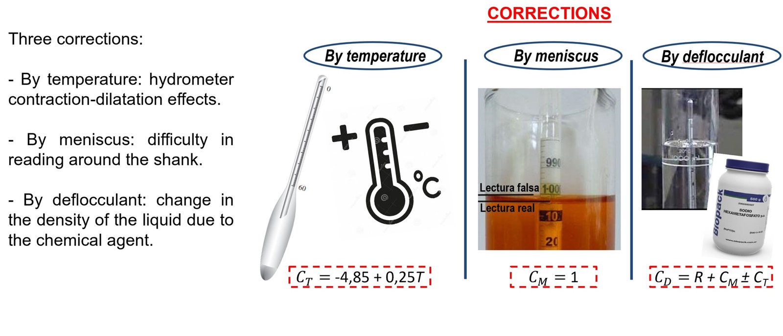
Figure 3 Corrections during the hydrometry test. In the figure CT = temperature correction factor; CM = meniscus correction factor; CD = deflocculant correction factor; R = reading taken on the hydrometer scale.
In order to obtain valid results during the test, it is essential to make the above-mentioned corrections accurately.
Uniformity and curvature coefficients
Once the information on the grain size distribution of a certain soil sample is complete, based on the sieving and hydrometer grain size tests, it is possible to analyze the resulting curve and determine two parameters of utmost importance for soil characterization: the coefficient of uniformity (cu) and the coefficient of curvature (cc). Figure 4 illustrates how to determine each.
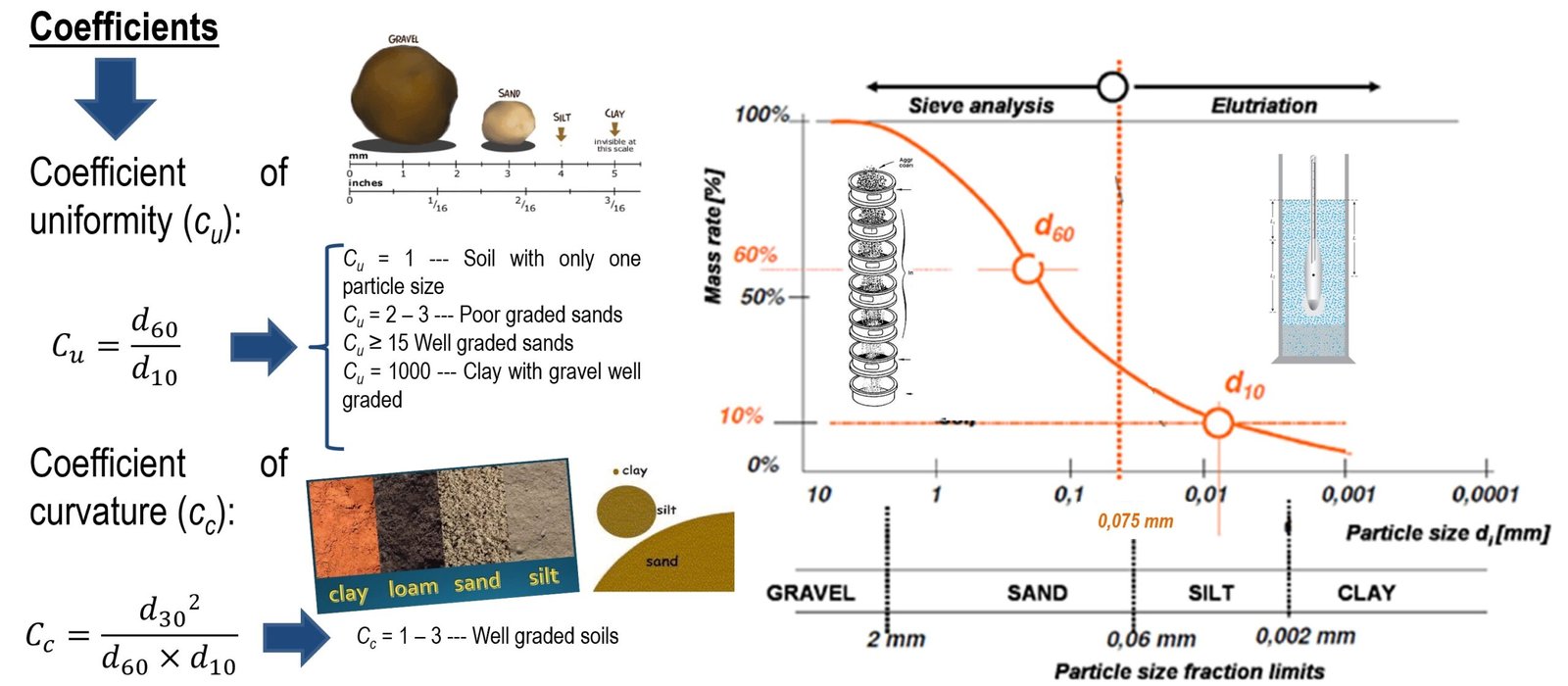
Figure 4 Coefficients of uniformity and curvature.
These two parameters are used in the Unified Soil Classification System (SUCS), which is the most widely used classification system around the world for geotechnical projects. Of these two coefficients, the most easily interpreted (and possibly the most practically useful) is the uniformity coefficient.
By relating the grain sizes d60 and d10, which are defined as shown in Figure 4, it is possible to determine how broad the curve is and, therefore, how broad the particle size distribution is in the sample.
Thus, the larger cu is, the more sizes the sample has, i.e., it is a well graded soil. If cu = 1, it means that d60 and d10 are equal, so you would have a sample with a single grain size (of course, such a sample does not exist, but it is good to imagine it to understand the concept).
It is important to note that the scale of the abscissae is logarithmic in all granulometric curves. This is something that allows us to have an idea of the enormous variation of sizes that a soil sample can have: from particles up to 4" (gravels), to particles that cannot be observed with the naked eye, such as clays and some silts.
With this we close this post on the hydrometer grain size test. It is convenient to review the references shown below, in order to complement the information described here.
References
- Das, B. (2002) “Soil Mechanics Laboratory Manual”. Fifth Edition. Engineering Press, Inc. California, USA.
- Head, K. (1980) “Manual of Soil Laboratory Testing – Volume 1: Soil Classification and Compaction Tests”. Pentech Press. London, UK.
- Mitchell, J.K. & Soga, K. (2005) “Fundamentals of Soil Behavior”. Third Edition. John Wiley & Sons, Inc. New Jersey, USA.